Getting Started with the NeuroPype Suite
Setup
For downloads and installation, see the introduction page.
License
Activating your License
When installation is completed, the Neuropype server application will start automatically. If it's your first time running Neuropype on that computer, you will be prompted to activate your license. A dialog box will pop up asking for your Intheon/Neuropype username and password. These will be the email address and password that you used to create an account on neuropype.io and purchase a Neuropype license (or obtain a free license in the case of the Academic edition).
You can view your license by logging into your account page. If you have the Startup Edition, you may cancel your license or add/remove seats on your account page online.
Changing your license
Upon installation, Neuropype saves your license information in a file called license.ini that is stored in the .neuropype\Neuropype <Edition> Suite folder of your user folder. So for example, if you have the Academic Edition and (on Windows) your username is Harry, your license.ini file is stored at c:\Users\Harry\.neuropype\Neuropype Academic Suite. If you need to re-input your license information for some reason, such as if you want to assign the Neuropype installation on a computer to a different user, simply delete the license.ini file. Restart Neuropype and you will be prompted for a license username and password. Enter the new username and password and, providing it is valid, your Neuropype installation will be assigned to the new user (and a new license.ini file created). Important: do not attempt to edit the license.ini file as this will cause the license check to fail. If you do edit it by mistake, then delete the file, restart Neuropype, and you will be prompted for your license info again.
Applications
The NeuroPype server
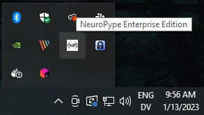
Once you have installed the suite and activated your license, the NeuroPype server will be running in the background, which you can see from the small NP icon in your Windows taskbar (lower right-hand corner of the screen; depending on your Windows setup, you may need to click the ^ in the taskbar to show the NP icon 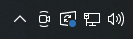 ).
).
Neuropype consumes relatively few resources and does not need to be turned off in most cases, but you can always right-click the icon and choose Exit to terminate it if desired. You can then bring it back up later from the Neuropype desktop icon. Note that you will not be able to run any data processing when the server is not active.
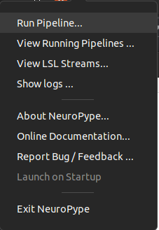
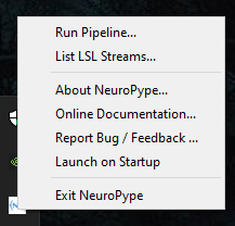
Right-clicking on the Neuropype icon will reveal a number of actions which you can take, including running a pipeline, seeing running pipeline, accessing help forums, etc.
The Pipeline Designer
The NeuroPype Suite includes a separate open-source Pipeline Designer application, which you can use to design, edit, and execute NeuroPype pipelines using a visual 'drag-and-drop' interface. You can launch the Pipeline Designer from the start menu under Windows or on other platforms as per the installation instructions for your platform. This will bring up the welcome screen (pictured below) where you can create or open a new processing pipeline.
Visit Working with Pipeline Designer for more information.
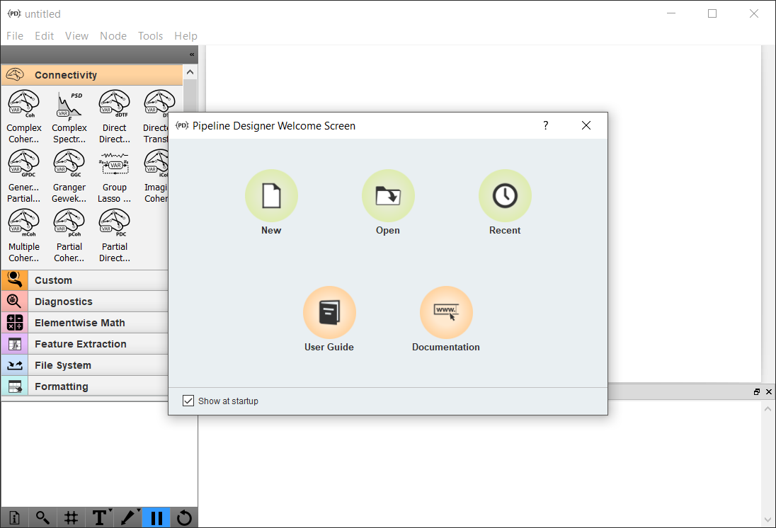
(Note that some of the widgets visible on the screenshots in this documentation may not be available in all editions of the NeuroPype Suite.)
The Experiment Recorder
The Experiment Recorder is a cognitive task presentation application that also uses Neuropype to capture LSL streams and record to disk. It is included in the NeuroPype Suite and can be launched from the start menu under Windows or on other platforms as per the installation instructions for your platform.
You can launch Experiment Recorder from the desktop application shortcut (Windows) or with Experiment\ Recorder/er.sh (Linux). See the Experiment Recorder documentation for more information.
Running your first pipeline
In this user guide, we'll take you through opening, editing and configuring a pipeline in Neuropype and explain the various aspects of working in Neuropype along the way.
While this website contains a great deal of documentation related to NeuroPype, the best way to become familiar with Neuropype is to load and run the example pipelines that ship with the software. These are found in the Examples folder of your installation, and can be opened with Pipeline Designer (see below). All the example pipelines will run out of the box with the example data files that ship with NeuroPype, but you can easily modify them to take live data from your own EEG headset or other sensor hardware, allowing you to get up and running quickly with your own data and perform a wide range of processing actions right out of the box.
Opening A Pipeline
To open one of the example pipelines that ships with NeuroPype, launch Pipeline Designer, select File | Open and navigate to the Examples folder inside your installation folder (e.g., C:\Program Files\Intheon\NeuroPype Academic Suite\Examples). For example, opening the file Bandpower.pyp will bring up a screen similar to the following:
: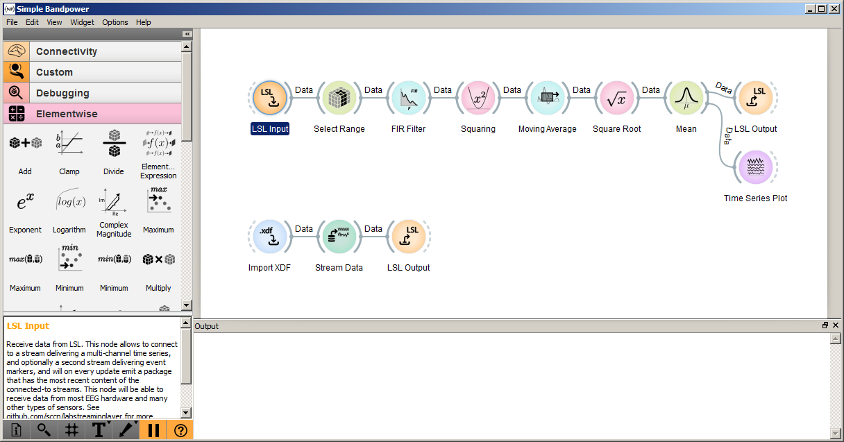
The large white area in the above screenshot is the 'canvas' that shows your current pipeline, which you can edit using drag-and-drop and double-click actions. On the left you have the widget panel, which has all the available widgets or nodes that you can drag onto the canvas. You can hover the mouse over any category or widget and see a tooltip that briefly summarizes it. The small box below is the help panel, which shows additional documentation for the current selected widget -- this will be your primary source of documentation for each node, and it usually contains far more information about a node than the small window may suggest. Below the help panel is the toolbar with the main actions buttons, most importantly pause/unpause. The empty white rectangle at the bottom right is the output window. This may not yet be open at first run, but by default it will pop up when the first output is displayed. You can either dock to the bottom of the canvas as shown in the above screenshot, or keep it as a free-floating window that you can, for instance, place on another screen.
Start Processing
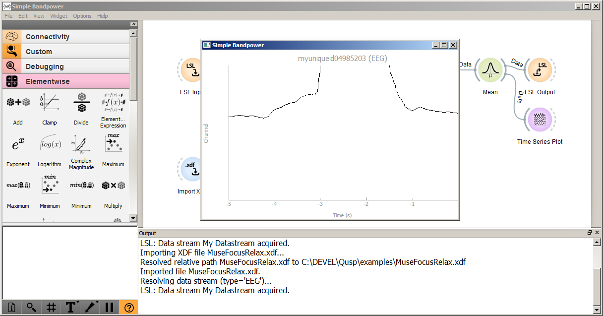
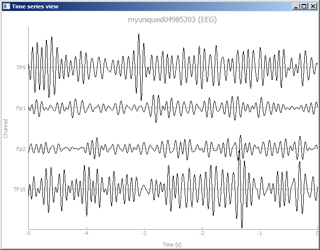
Click the play icon in the toolbar to start running the pipeline. When you do, Pipeline Designer will send an API call to the NeuroPype server to instruct it to begin executing the pipeline. You will see log messages in the output window, and after a few seconds, it will show a time series view similar to the following (visual details may differ depending on the release). Your first signal processing pipeline is running (congrats!).
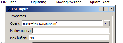
Note that, if there are multiple EEG streams on the network currently via LSL, this pipeline may pick up the first one that it finds, which may not be what you expect (if so, you can double-click the LSL Input node and change the first entry to name='My Datastream' as shown below):
Pipeline Info/Docs
You can query information about the current pipeline by clicking the info toolbar button (with the i icon):
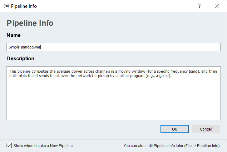
For more complex pipelines this info will contain generally useful information, so don't skip it! (See also node documentation below.)
Changing pipeline settings
Changing Node Settings
You can change the settings of any processing nodes in your canvas by double-clicking on it. For instance, when you double-click on the Import XDF node, a window pops up that shows you the settings (including the file name to import).
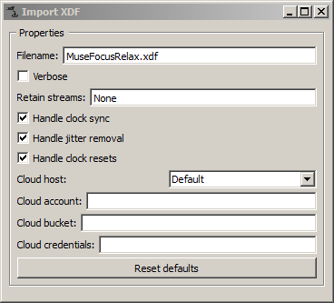
When you edit a setting of a node (e.g., the filename), it will be instantly applied, and the processing behavior of the pipeline will change (if it's currently unpaused). If you need to edit multiple settings at once, it's a good idea to pause the pipeline before making the changes to avoid crashes because of inconsistent settings. The Import XDF here is importing a file containing a few minutes of data from a 6-channel InteraXon Muse EEG headset (during the recording, a person was alternatively focusing and relaxing to make it more interesting).
Node Documentation
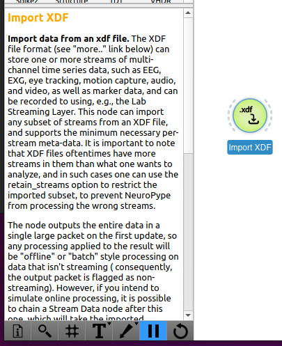
When you click on a node in the canvas (on or in the sidebar showing all the nodes), the documentation for that node will be shown in the bottom right-hand corner of the screen. This explains the overall purpose of the node and any special behavior to be aware of (such as what type of input it expects or output it generates, whether it works with recorded (i.e., "offline") or streaming (i.e., "online") data, etc.).
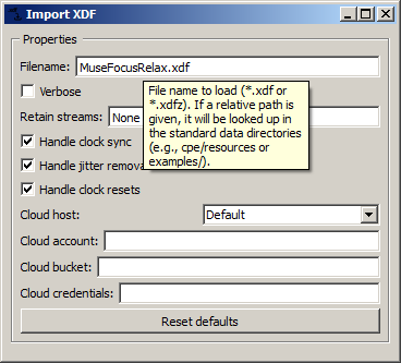
In addition, documentation about each node's settings is available by hovering over a setting in a node's settings window (opened by double-clicking a node in the canvas). A tooltip will appear with detailed information about the setting. In the image below, the reason the file is found, even though the path is not omitted, is that it's in the Examples/ folder that comes included with the suite.
This same node and node settings documentation is found online in the Nodes section of this website.
How a pipeline works
Data Flow Basics
When you execute a pipeline in NeuroPype, the data flow behaves as follows. It is really quite simple: generally, data exits a node on the right side along the grey wire and continues to the next node, gets processed by it, and then exits that node along its output wire on the right, and so on. Data generally flows from left to right through a node, as shown below.
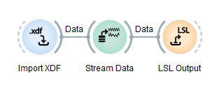
In this pipeline, the import node has no input wire since it's a data source. It loads the given file, and then outputs it via its output wire. That file then travels into the Stream Data node where it's stored in memory and subsequently streamed out in real time to the next node. The LSL Output node takes that real-time data stream and broadcasts it out over the LSL network (LSL=Lab Streaming Layer, see this video), where it can be picked up by other programs on the computer/LAN/Wi-Fi (e.g., a game), or by the same program.
The interesting thing to note here is that the output of the Import node is the entire recording, i.e., a very long chunk of data, which is also called offline (or batch) processing, while the output of the stream data node and input to the LSL node are small successive chops of the data comprising a real-time stream, often only 100ms or less in length. This is also called online processing. As showcased by this simple pipeline, the data flow engine of NeuroPype can easily do both in the same pipeline.
Ticking
NeuroPype does online processing as follows. When NeuroPype is running your pipeline, it will periodically perform a tick (by default 25 times a second) unless you pause it. In each tick, it will go through your pipeline in data flow order (in this example pipeline, it's left to right, top to bottom), update each node in turn, and move whatever data is produced by it through its output wires into the inputs of the next node (then update that node, move its output data to the subsequent node, and so on). This order is called topological order, and it doesn't depend on where nodes are on the screen (just on how they are connected).
Data and Data Sources
The data that travels over the wires may be an entire recording (e.g., what is produced by Import XDF and accepted by Stream Data), or it may be just a small chunk of data of some ongoing 'live' data stream (e.g., what is produced by Stream Data and consumed by LSL Output). Generally, the Import nodes will output the content of the entire data file in one large packet, and will output nothing on subsequent ticks. Input nodes in the Network category (see list of categories in widget panel), such as LSL Input, will return whatever was received since the last tick (which would usually be a small chunk). If you are doing offline processing, in general you can reset/reload the pipeline by clicking the rightmost button in the toolbar (the circular arrow in your GUI) to re-run any offline processing. Note that some screenshots of this guide show a question mark icon instead (this is from a previous version).
Processing Nodes
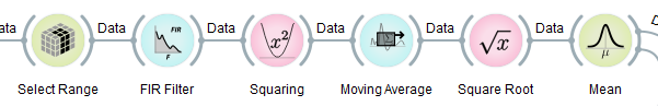
Most of the nodes offered by NeuroPype are processing nodes, such as those shown below (from the upper chain in the SimpleBandpower pipeline). These nodes accept a packet, and output a processed packet, and if they receive a whole recording, they will output a whole recording, and if they receive a small chunk, they will output a small chunk.
Some exceptions to this behavior are the Stream Data node that we discussed before, whose jobs are to take a recording and then chop it up into many small chunks which are output over multiple successive ticks (i.e., real-time playback). Other exceptions are special-purpose nodes that may, for instance, buffer a certain amount of streaming data until a condition is met, and then output it in one large chunk (e.g., nodes that need to see a minimum amount of data to calibrate themselves on it). Ideally you should go through the help text of each node (in the help pane) to see how it behaves. Many of the nodes serve very special purposes, and may require data to be in a specific form to work as intended. You will generally find a lot of information on this in the node's help text in the help panel.
Output/Visualization Nodes
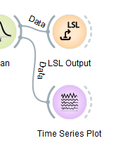
Some nodes act as 'data sinks', i.e., they take in data but have no outgoing wires. Their functions include file export, transmission over the network, and visualization, e.g., like the two nodes at the end of the upper chain in our pipeline (one sending the data over the LSL network, and the other plotting the incoming data as a streaming time series).
Adding nodes to your pipeline
Adding New Nodes
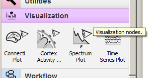
Let's peek into the data stream between the FIR Filter node and the Squaring node. For this, you can scroll the widget panel down to the Visualization category and click on it to expand its contents as below:
Now you can grab the Time Series Plot node with the left mouse button and drag-and-drop it under the Squaring node.
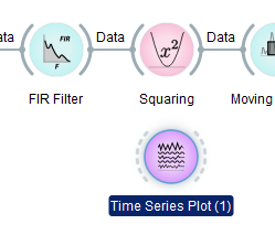
Now you can left-click on the grey arc on the right of the FIR Filter node, hold the button, and drag a wire to the dashed arc on the left of the Time Series Plot (1) node, and release.
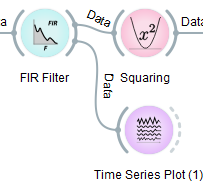
As a result, a second time-series plot will open itself (if the pipeline is unpaused) and show 4 channels. Note that, on some versions of Windows, new plots may open behind the Pipeline Designer window, but they will be highlighted in the taskbar for easy discovery. You can press the '-' key on your keyboard in order to change the scale of the signal.
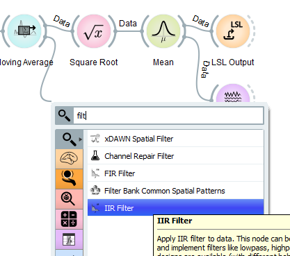
Tip: you can also add nodes by dragging a wire out from one node and then releasing it somewhere over the blank canvas. This will bring up a context menu with a categorized list of nodes that you can insert; you can even start typing, and it will prune the list to show the nodes that contain the substring you typed.
Data in Neuropype
Data Packets
In simple pipelines as this one, the data packets that travel along your wires on each tick are all multichannel time series (i.e., each is a 2D array of channels by time-points). However, in more sophisticated pipelines, you can have data that are 3D arrays, for instances multichannel time-frequency diagrams, or arrays of even more dimensions, such as the data that is flowing in pipelines that deal with brain connectivity measures. General n-way arrays in NeuroPype are called tensors.
Tensors in NeuroPype are not just a grid of raw numbers, but in fact each of the axes has a type (e.g., time, space, frequency), and stores information about the scale (such as the time range in seconds for a time axis). Some axis types also have labels (for instance, channel labels, feature labels, or trial labels). It is for this reason that the above plot is able to plot both the channel labels and the time correctly, or that a frequency spectrum plot would show the correct frequency axis. These axes can be compared to column or row headers in a table, though they can hold more than one piece of information (for example, the Space axis can hold multiple pieces of information about each channel, such as its label, 3D positions, unit, etc.).
Lastly, the data stream can have other meta-data attached to it (referred to as Stream properties or props in Neuropype), such as the provenance (what device or file it came from), the data modality (for instance, EEG, shown on the top), and so on.
In short: In Neuropype data is passed between nodes in Packets. Each Packet contains one or more Streams. Each Stream contains a block made up of an n-way tensor (typically referred to as data in Neuropype nodes, or if you write your own nodes, this would be the block.data), and axes which describe the rows/columns of that data.
Multiple Streams
Sometimes you have multiple pieces of data that you would like to transmit together side by side. One example of this is EEG and EOG coming from two different amplifiers. Another example is having EEG plus event markers, and some more examples are having simultaneous data from N subjects in a group experiment, or features plus labels in machine learning. Sometimes these different pieces of data are best treated independently, e.g., when you want to apply different kinds of filters to each, and in that case you can have parallel data paths in your pipeline, each with its own processing nodes. However, in NeuroPype multiple streams can also be bundled together and transmitted together over a single wire. Many nodes can naturally produce multi-stream packets, for instance importing or exporting an EEG file that has both EEG and markers, and there are special nodes to bundle and your data streams as you wish (look for nodes with "Stream" in the name). For example, the Merge Streams node allows you to combine streams from different sources (i.e., two different LSL inputs) into a single packet for processing, while Extract Streams provides the opposite function (separating streams for operating on a single stream only, for example a stream containing ECG data on which you wish to perform cardiac-related functions).
"Offline" (recorded) vs "Online" (streaming) data
Neuropype can process both streaming ("online") and recorded ("offline") data. See Offline vs Online data for more details on this.
Signal Processing
NeuroPype has a lot of signal processing nodes (the Pipeline Designer shows these under the Signal Processing category), for instance the FIR Filter node, which is one of the most useful of them and whose settings are shown below.
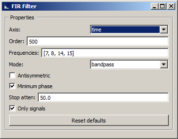
This node as used here will perform a band-pass filter, and retain only the 8-14 Hz frequencies. However, often the rolloff at the band edges is not very sharp (since that would be difficult to realize with a low-order filter), and only frequencies outside 7 and 15 Hz are fully attenuated (the 1 Hz transition bands are partially attenuated). When you change these frequencies, it's good practice to not make the band edges unnecessarily steep. In addition, you can try to reduce the order of the filter (especially if you band edges are loose and if your cutoff frequencies are high), but note that the filter can end up leaking frequencies outside those bands, which can, for instance, cause slow drifts that can break all sorts of subsequent signal processing. A very high order will drive up your CPU usage and can slow down processing. You can also try the IIR Filter as an alternative (though make sure you read up on the principles behind it). You can play with the frequency parameters of this filter and watch how the signal changes that the time-series viewer that you added is plotting.
Another very important node is the Select Range node, which allows you to select a subset of the data that passes through the node -- make sure you read the help text and tooltips to understand how it operates. For instance, you can select data along any axis, here space (channels), and the selection can be a range, such as 1...5, or a list of indices (e.g., [0,1,2,3]). There is also a Python-style syntax that uses colons, where 2:7 goes from 2 to 6, but, unlike MATLAB, this syntax does not include the last element in the range. The setting in this pipeline removes the last 2 channels, since they happen to contain digital garbage, which can pollute the visualization if not removed; if you use a different dataset or headset, you will have to change this to remove a different set of garbage channels.
The last three processing nodes compute the sliding-window root-mean-square power of the signal (in the frequency band that the FIR filter retains), and finally averaged across all channels.
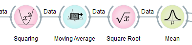
The 8-14 Hz band is also known as the 'alpha' frequency band in EEG, which primarily picks up idle activity of neurons in the brain. That is, when one relaxes and/or closes the eyes, the alpha power, which is computed by this filter chain, will go up, and that's why this pipeline computes a very simple relaxation measure.
Getting data in and out of Neuropype
Lab Streaming Layer
You might be asking how the signal makes it from the import node to the FIR filter node, because there is no wire between the two nodes. The reason is that, in between the LSL Output node at the bottom of the patch and the LSL Input on the top left the data travels invisibly over the LSL network. LSL works even between different computers on the same WiFi or LAN, i.e., if the LSL output node was on one PC and the LSL input node was placed in a second pipeline that you have open on another PC, data would flow from one to the other in just the same way (unless you computer's Firewall gets in the way). Since there could be many inlets and outlets present on a given WiFi or LAN, there could be quite some confusion, and therefore the outlet generally assigns a unique name to the stream, while the inlet is set to look for a stream with that particular name on the LSL network.
LSL is not only a way to get data from one computer to another, but also to get data from your EEG system, or any other kind of sensor that supports it, into NeuroPype. You can also use it to get data out of NeuroPype into external real-time visualizations, stimulus presentation software, and so on.
This pipeline uses LSL simply to make it very easy for you to switch from playing back pre-recorded data, which is what this pipeline is doing, to processing data from a live EEG system. All you have to do is delete the three nodes at the bottom, and then tell the LSL Input node to read from your EEG amplifier instead.
Using LSL
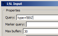
LSL is the easiest way to get live sensor data into NeuroPype, and is widely supported by many biosignal device hardware makers. If you have a sensor that is supported by it (see https://labstreaminglayer.org/), then you only need to get the sensor, start the acquisition program, enable LSL streaming in that program (or for some sensors, start additionally an LSL client that translates the acquisition program's output to LSL), and make sure that the LSL Input node has a query string that matches that sensor. For instance, if you use type='EEG' as below, then you will pick up data from the first EEG device on the network that it finds:
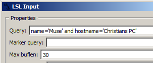
... this is fine if you're testing this at home, but if you're at a public place where others may be running their own LSL streams (or perhaps you are running more than one stream, such as one playback and one actual device), you must be more specific than this. For instance, you can refine the search using the name of the stream, as in name='Cognionics Quick-20' to read from a specific Cognionics headset. But if there are more than one headset of that type in use on the network, you won't know which one you're reading from -- in this case, it's best to include your computer's hostname, as well, as in the following example:
As a side node, when you change the LSL stream, you may well end up with a different number of channels (or sampling rate, etc.), than what you had before in the playback data, and when you do that while the pipeline is running, some nodes may be unprepared for that switch. Think of it like changing engine parts of a moving Formula 1 car. You can do a lot of changes while the pipeline is running, but if you do encounter an error, you can click the reload button (the circular arrow next to pause/unpause) to reset the pipeline back into a healthy state. Note that any state that the pipeline may have accumulated (such as buffers or calibration) is cleared by this action, as well.
Using Vendor-Supplied Software
How data from a sensor gets into LSL depends on the specific sensor, as mentioned before -- a good starting point is to download the latest LSL distribution from https://github.com/sccn/labstreaminglayer (which also includes some useful debugging utilities), check whether any matching app is included for your hardware, and if not, check if the vendor hardware happens to have LSL support. There is also a fairly recent copy of an LSL distribution included with the NeuroPype Suite. Or alternatively you can check if your vendor happens to support LSL natively, which many of them do. For instance, in the case of the Muse, a program called muse-io (shown below) is included by the vendor.
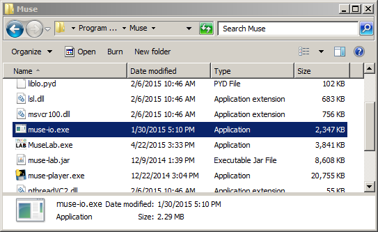
This program can be invoked from the command line to stream out over LSL, as shown below:
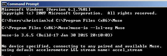
In this case you can give the stream a name yourself (we used 'Muse' here) which allows you to disambiguate your stream from others that may be on the network, but most vendors will hard-code the stream name.
For more detailed information on the use of various hardware with Lab Streaming Layer please see this section.
Viewing available LSL streams
You'll often find it useful to see which LSL streams are present on your network (whether created by Neuropype or by some other application such as a device hardware vendor app). There are two ways to do this:
- In Pipeline Designer, select the
Tools,View LSL Streamsmenu item. A window will pop up with the LSL streams on the network, including the LSL stream name, type, number of channels, hostname (i.e., it may have been created by another computer on the network), and streamID.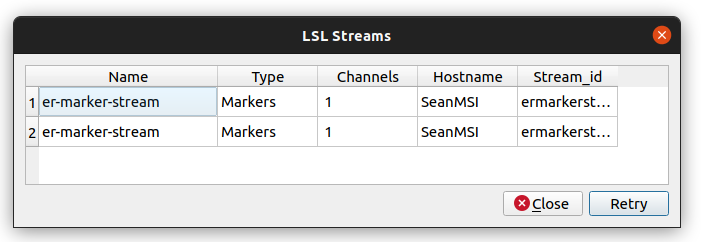
-
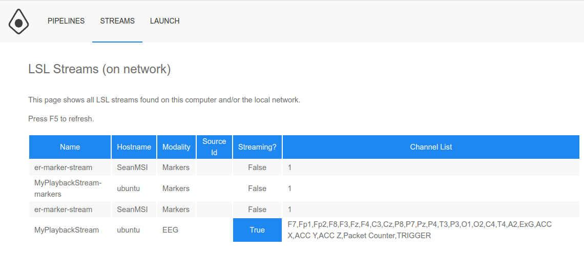
Select the
View LSL Streamsfrom the Neuropype menu (in the Windows taskbar) to open the Neuropype Control Panel; or if you already have the Neuropype Control Panel open, click on theSTREAMSmenu item. In addition to the information shown when viewing the streams from Pipeline Designer, you can also see whether a stream is presently streaming data (remember a stream remains active even if it is not presently streaming data, until it is closed or the pipeline execution that created it is deleted).Note that it takes a second for the Streams page to come up as it checks the LSL streams to see whether they are streaming any data.
Biosignal processing in Neuropype
To get started with running your first pipeline, head over to see some common biosignal processing operations in Neuropype. For some more information on Neuropype features, see below.
Neuropype menu actions
Neuropype runs as a background service and can be accessed by other applications, such as Pipeline Designer, or your own apps, through its API. (See the Developer documentation for details on this.) Neuropype consumes very little resources while at rest, so you can safely leave it running all the time. You can easily interact with Neuropype through the Pipeline Designer, but Neuropype has some functions that can be accessed directly.
When Neuropype is running you will see an NP icon in your system tray. Right-clicking on that icon will bring up a menu of actions, described below.
Run pipeline
This will bring up the Neuropype Control Panel, a local web application that runs in your browser and which allows you to select, configure and run a pipeline on your computer. It's an easy alternative to Pipeline Designer for cases where you don't need to edit a pipeline. Any pipeline settings exposed using the ParameterPort node will be available to modify in the client before running the pipeline.
The Neuropype Control Panel also shows you which pipelines are currently running, and allows you to pause, resume, or stop them.
List LSL streams
This links to a page in the Neuropype Control Panel showing all LSL streams found on your computer and network. Useful for seeing which streams are actually present when trying to capture on for your pipeline. Note that the Tools | View LSL Streams menu item in Pipeline Designer provides similar functionality.
About Neuropype
Shows the Neuropype edition and version. Also links to the Neuropype EULA and the licenses for open source software used in Neuropype (i.e., Python, numpy, etc.).
Online documentation
Links to this website.
Feedback and Bug Reports
We appreciate your reports on any bugs that you encounter or questions about how to use certain nodes that are unclear, or any other feedback that you may have. Do to so, simply use the Report Bug / Feedback link available in the Neuropype menu (available by clicking on the Neuropype icon in your system tray). This will take you to the Discussions page of the Neuropype website where you can create a post (you'll be prompted to log in with your Neuropype credentials if you aren't already).
Launch on startup
On installation, Neuropype is set to launch automatically when you start Windows. You can disable that by unchecking this menu item.
Exit Neuropype
Exits Neuropype and terminates all Neuropype processes. At this point, neither Pipeline Designer nor any other client application will be able to connect to Neuropype. (Pipeline Designer will run but not show any nodes, since those are provided by Neuropype.) Mostly useful for cases where you need to restart Neuropype.
Neuropype Usage Tips
Click here for the Tips & Tricks section of our only forums where we post tips and short tutorials on how to perform certain tasks with Neuropype. We regularly add new posts (often taken from generally applicable support questions in the forums), so it's a good place to look when you have a question. See also the Neuropype Tutorials in this documentation.
Neuropype Experiment Recorder
Visit the Experiment Recorder page to learn how to use the Experiment Recorder to easily present cognitive tasks and record data from LSL streams to disk. Together with Neuropype, ER provides a complete solution for experiment presentation, data collection, and data analysis.
Copyright (c) Syntrogi Inc. dba Intheon. All Rights Reserved.