Biosignal processing in Neuropype

On this page we will briefly tour a few common biosignal processing functions in Neuropype. (With over 400 nodes in Neuropype, there is an almost infinite variety of pipelines that can be built; this page only covers a small fraction of the more common ones for EEG.)

We've included a number of example pipelines in your Neuropype installation, and loading, running, and adapting them is one of the best ways to get started with biosignal processing. You'll find these in the Examples folder of your installation, and can open, copy, edit and save them using Pipeline Designer.

Using Artifact Removal

Most robust EEG processing pipelines require some sort of artifact removal. NeuroPype has a number of processing nodes for this job, for instance the Channel Repair node shown in the below graph, which you can open by loading the file ArtifactRemoval.pyp in the Examples folder.

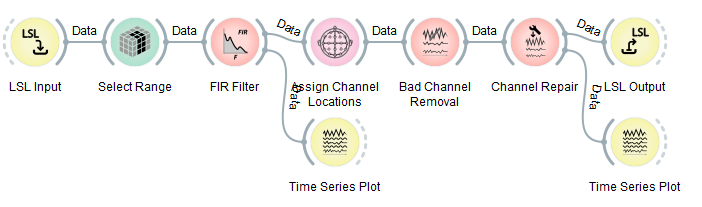
Be sure to inspect the settings of these nodes when you want to add EEG artifact removal to your own pipeline, and also make sure you visually check the quality of the artifact removal using some time series plots as done here to ensure that your settings are good. You need to remember the following things: (1) you need to remove garbage channels beforehand (done here by the Select Range node, which is here set to keep the first 4 channels, since this example was written for the Muse). (2) you must have a decent high-pass filter before artifact removal that reliably removes drifts (here this is an FIR filter with a sufficiently high order, at least 50db suppression, and 0.5 to 1Hz transition band). If your sensor has enormous drifts, you may need to increase the suppression and/or order. (3) then come the artifact removal nodes, which work only on EEG, not on other kinds of signals. (4) these nodes are adaptive, and they must first see a certain amount of data, e.g., 20 seconds, in order to calibrate themselves.

Online Calibration

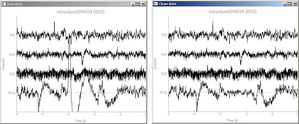
These nodes will first buffer up several seconds of data until they have enough (during that time the graph swill output nothing), then it calibrates itself, cleans the data that it has buffered, and sends it out as one big chunk; once that's happened, the nodes will clean and pass through any subsequent small chunks that they get (i.e., operate in real time). While the nodes are collecting calibration data, you will see only one plot showing the raw data streaming, but once they are calibrated, a second plot will open up and shows the clean data next to it, as below.

Accumulating Calibration Data for Machine Learning

Next we will discuss machine learning (specifically supervised learning). If you're not familiar with that, or have no intention to use it at this point, you can skip or gloss over these sections. The machine learning nodes in NeuroPype are also adaptive, but unlike artifact removal, they will not simply buffer up the first few seconds of session data on their own (because that data for calibration must meet certain conditions, for instance it must include labels). Instead, we place a special node early in the pipeline whose job it is to buffer up the calibration data, and then to output it in one big chunk that travels through the rest of the pipeline, causing each subsequent node to update (and calibrate) itself accordingly. From then on, subsequent data packets pass through the graph normally, and all nodes (now calibrated) can transform the raw inputs into predictions as they should. This special node is called Accumulate Calibration Data.

Imagined Movements Classification

The use of that node is shown in the file SimpleMotorImagery1.pyp, which you should now open. The pipeline should look as follows:

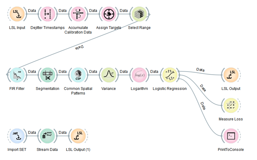
This pipeline can predict from EEG whether you're currently imagining one of multiple possible limb movements (default: left hand movement vs. right hand movement, a.k.a., two-class classification). The output of this pipeline at any tick is the probability that the person imagines the first type of movement, and the probability for the second type. Note that this pipeline prints its output to the NeuroPype console. If you are not seeing the console, you can open it from the Options menu by selecting Show Output View. You will almost certainly want to dock the output view to the bottom of the VPE canvas by grabbing the title bar and dragging it over the bottom 10% of the canvas, at which point a visual dock indicator appears, and releasing.

Since the EEG patterns associated with these movements look different for any two people, several nodes (here: Common Spatial Patterns and Logistic Regression) must first adapt themselves based on some calibration data for the particular user, and moreover, it's not enough for the calibration data to be some arbitrary EEG but must meet certain criteria as we already alluded to earlier (while we show it here for imagined movements, the same rules apply to pretty much any use of machine learning on EEG). First, the node needs to obtain example EEG of left-hand movement and example EEG of right-hand movement, respectively. Also, a single trial per class of movement is far from enough, rather the node needs to see closer to 20-50 repeats when you use a full-sized EEG headset. And lastly, and these trials also must be in more or less randomized order, i.e., not simply a block of all-left trials followed by a block of all-right trials. Collecting data in that way is one of the most common beginner mistakes with machine learning on time series, and it is important to avoid it, even if it means collecting some new data.

Working with markers

EEG Markers

For the aforementioned reasons, the EEG signal must be annotated such that one can tell at what points in the signal we have example data for class 1 (person imagines left hand movement) and where we have example data of class 2 (right hand movement). One way to do it is to include a special 'trigger channel' in the EEG, which takes on pre-defined signal levels that encode different classes (e.g., 0=nothing, 1=left, 2=right). While NeuroPype can parse trigger channels (by inserting a Parse Trigger Channel node just before the Accumulate node), this pipeline does not use them.

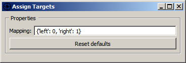
Instead, the pipeline assumes that the data packets emitted by the LSL Input node have not just one stream (EEG), but also a second stream that has a list of marker strings plus their time stamps (markers), i.e., they are multi-stream packets and there are consequently two data streams flowing through the entire pipeline. The markers are then interpreted by the rest of the pipeline to indicate the points in time around which the EEG is of a particular class (in this pipeline, a marker with the string 'left' and time-stamp 17.5 would indicate that the EEG at 17.5 seconds into the recording is of class 0, and if the marker had been 'right' it would indicate class 1). Of course the data could contain any amount of other random markers (e.g., 'recording-started', 'user-was-sneezing', 'enter-pressed'), so how does the pipeline know what markers encode classes, and which classes do they encode? This binding is established by the Assign Targets node, whose settings are shown below (the syntax means that 'left' strings map to class 0, 'right' maps to class 1, and all other strings don't map to anything).

Segmentation

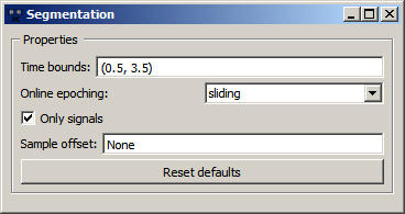
The second question is, given that there's a marker at 17.5 seconds, how does the pipeline know where relative to that point in time we find the relevant pattern in the EEG that captures the imagined movement? Does start a second before the marker and end a second after, or does it start at the marker and ends 10 seconds later? Extracting the right portion of the data is usually handled by the Segmentation node, which extracts segments of a certain length relative to each marker. The below graphic shows the settings for this pipeline, which are interpreted as follows: extract a segment that starts 0.5 seconds after each marker, and ends 3.5 seconds after that marker (i.e., the segment is 3 seconds long). If you use negative numbers, you can place the segment before the marker.

Accumulation

The third node in the top row is our accumulate node. Double-click it to inspect the settings:

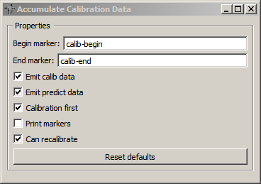
The most important detail here are the Begin marker and End marker fields: this node assumes that the beginning and end of the period in the data stream that contains calibration data is identified by markers in the data stream, and these two fields let you choose which marker strings the node is looking for. So in summary, the pipeline expects that your data stream has at some point a marker string named 'calib-begin', followed by a bunch of 'left' and 'right' markers in pseudo-random order, followed by a 'calib-end' marker.

Calibration Marker Generation

So now you want to calibrate the pipeline: how do you get the markers into your EEG stream? If you're using a pre-recorded file (e.g., the example file that the pipeline is loading and playing back in the bottom three nodes), then the required markers are hopefully already in the file (in this case we made sure they are). However, if you're working live, i.e., you're wearing an EEG headset, how do you generate the markers live? This is actually again very easy using the lab streaming layer: basically you need a script (for instance, in Python, MATLAB or C#) that calls an LSL function like send_marker('left') -- have a look at the examples at https://github.com/sccn/labstreaminglayer/wiki/ExampleCode.wiki (look out for examples titled "Sending a stream of strings with irregular timing" or "Sending string-formatted irregular streams" for the language that you're using). For instance, here's how to send a marker in Python:

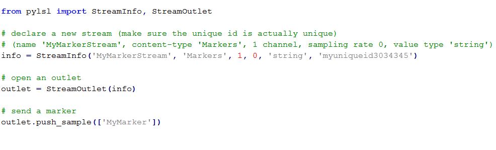
Of course a real program would send all the markers, and since those need to match what the person is imagining, it would basically manage the entire calibration process and instruct the user when to imagine what movement (that's also where the 0.5 and 3.5 in the segmentation node come from -- it takes about half a second for a person to read the instruction and begin imagining the movement, and he/she will finish about 3 seconds later and get ready for the next trial). Here is a very simple script that print L or R to indicate when a person should imagine the movement and simultaneously sends a left or right markers to an LSL stream:

import time
import random
from pylsl import StreamInfo, StreamOutlet

warmup_trials = 10
trials_per_class = 60
perform_time = 3.5
wait_time = 1
pause_every = 30
pause_duration = 10
labels = ['L', 'R']
markers = ['left', 'right']

info = StreamInfo(name='MotorImag-Markers', type='Markers', channel_count=1,
                  nominal_srate=0, channel_format='string',
                  source_id='t8u43t98u')
outlet = StreamOutlet(info)

print("Press [Enter] to begin.")
x = input()

for trial in range(1, warmup_trials+trials_per_class*len(labels)+1):
    choice = random.choice(range(len(labels)))
    print(labels[choice])
    if trial == warmup_trials:
        outlet.push_sample(['calib-begin'])
    if trial > warmup_trials:
        outlet.push_sample([markers[choice]])
    time.sleep(perform_time)
    time.sleep(wait_time)
    if trial % pause_every == 0:
        print('Pause')
        time.sleep(pause_duration)
outlet.push_sample(['calib-end'])

If you want to throw machine learning at other prediction tasks, e.g., workload, you would also author a corresponding calibration program that, for example, puts the person into high workload (for instance by setting the game difficulty to high) and emit, say, a 'high' marker into LSL, and then puts them into a low workload state and emit a 'low' marker, and so on. Or to calibrate emotion detection you could try to play happy vs. sad music, and so on.

Picking up Marker Streams with LSL

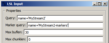
The LSL Input node is responsible for returning a marker stream together with the EEG. For this to happen, it first needs to find and pick up that stream on the network, of course. The name of the marker stream that it should look for can be entered in the second settings field, named Marker query (or it can also be a compound expression to ensure that it's uniquely identified on the network, similarly to the example earlier under Using LSL):

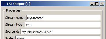
The LSL Output node used to send out the data which is being played back by the Stream Data node at the bottom of the pipeline is set up to send out not just the EEG stream, but also a marker stream:

So in summary, the data file that's being imported by the Import Set node contains 2 streams (EEG and markers), which you can also verify by importing that file into EEGLAB for inspection (if you have MATLAB). Then, this 2-stream recording travels into the Stream Data node, gets stored in memory, and then is being played back in real time and chunks of it are forwarded to the LSL Output node. This node creates 2 LSL streams, which are picked up by the LSL Input node, and then travel through the entire remainder of the pipeline. And if you delete the three playback nodes at the bottom, you need to have 2 live LSL streams, one from your headset and one from your app that controls the calibration process, in order to calibrate the pipeline. By the way, since the calibration session is actually over 15 minutes long, in this example the Stream Data node is set up to play back the data at 10x real-time speed, to shorten the wait time for you until something interesting happens (you can dial it back to 1x by editing the node settings).

Calibration

Using Pre-Recorded Calibration Data

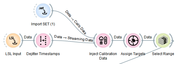
Our pipeline is doing a great job, but wouldn't it be nice if we didn't have to re-collect the calibration data each time we ran the pipeline? It's often more convenient to record calibration data into a file in a first session, and then just load that file every time we want to run our pipeline. This is actually quite easy, and for this the Accumulate Calibration Data node needs to be replaced by an Inject Calibration Data node, which has a second input port where one can pipe a calibration recording in (which we import here using Import Set). This is implemented in SimpleMotorImagery2.pyp, and the relevant section looks as follows (rest stays the same):

The imported calibration recording will be injected into the data stream on the first tick, and so it travels through the rest of the pipeline, all nodes can calibrate themselves properly based on it. After that, the regular real-time stream coming from the LSL Input node will flow through the graph and get transformed by it into predictions.

Recording Calibration Data

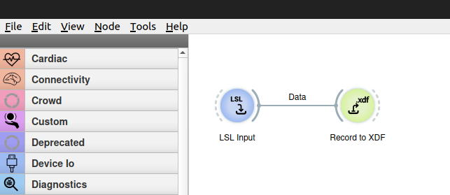
You can easily record calibration data by making a simple pipeline with an LSL Input and a Record To XDF node. This will capture data from the stream configured in the LSLInput node (put name=streamname in the Query parameter of the LSLInput node, or leave the default to capture the first EEG stream found on the network), and record it to the filename parameter specified in the Record To XDF node. (Remember that you can see which LSL streams are on the network using the Tools | View LSL Streams in Pipeline Designer).

Alternatively, you can use the LabRecorder program that comes with the LSL distribution included with Neuropype (see Lab Recorder documentation at https://github.com/sccn/labstreaminglayer/wiki/LabRecorder.wiki).

You can then use the Import XDF node to import the file you created and feed it into the Inject Calibration Data node.

More example pipelines

Check out the example pipelines in the Examples folder of your installation. You may find a pipeline that is already doing some or all of what you want to accomplish, or which you can adapt, and can save yourself building one from scratch.